The XLOOKUP function in Microsoft Excel is a powerful search tool, allowing you to find particular values from a range of cells. It acts as the replacement for earlier lookup functions like VLOOKUP, eliminating many of their limitations.
I’ll explain how to use XLOOKUP, step-by-step, in this tutorial.
As the name suggests, lookup functions like XLOOKUP pull matching data (exact matches, or the closest available match) from a dataset in Excel. If there’s more than one matching result, the first or last result in the set is returned, depending on the arguments used.
XLOOKUP acts as a custom search tool, flexible to the demands of different types of data in custom-built Excel spreadsheets. XLOOKUP is a relatively new function, only becoming available for Microsoft 365 users back in 2020. However, it’s quickly become one of the best Excel features for data analysis. If you’d like to start playing with data in Excel, have a go at our free 5-day data analytics short course to learn the basics.
Are you struggling to figure out XLOOKUP? In this article, we’ll explain:
- What is the XLOOKUP function and how does it work?
- How does the XLOOKUP function work in Microsoft Excel?
- Things to consider before using the XLOOKUP function in Excel
- How to use XLOOKUP in Excel: A step-by-step guide
1. What is the XLOOKUP function and how does it work?
Excel already has a number of tools for searching through data, from conditional formatting rules to the built-in find and select tool.
These features, however, don’t really change your spreadsheet in a meaningful way. You couldn’t easily reference a formatted cell by color in another formula automatically, for instance.
Why we need LOOKUP functions
What if you had data that you need to quickly search through, with custom search criteria that you need to change regularly?
This isn’t an uncommon scenario for data analysts, who might want to search and return individual results from a dataset with queries that can be quickly customized.
VLOOKUP and HLOOKUP—possible fixes
Postal addresses, classroom exam results, profit margins—if you want individual results from datasets like these, the best tool to use is a lookup function. Lookup functions are a staple of complex Excel spreadsheets, with VLOOKUP and HLOOKUP among the most common.
The problem with VLOOKUP (or vertical lookup) and HLOOKUP (horizontal lookup) formulas is that, as the elongated names suggest, they’re pretty limited in scope, forcing you to use workarounds to work with data to the left or right of values (among others).
The solution—XLOOKUP
You can bypass some of these limitations with other functions (like INDEX and MATCH), but the process isn’t efficient. XLOOKUP is the resolution to this problem, allowing you to look up data in columns and rows, both to the left or right of your search value.
It can handle approximate matches, multiple search values, nested queries (using multiple XLOOKUP functions in a single formula), custom error messages, and more. XLOOKUP is (at present) only available for Microsoft 365 subscribers, but for both basic and complex data searches, it’s an absolute game-changer.
2. How does the XLOOKUP function work in Microsoft Excel?
To explain the XLOOKUP function properly, we’ll use an example scenario. An example Excel spreadsheet contains the staff list of a small company, containing IDs, names, email addresses, and responsibilities.
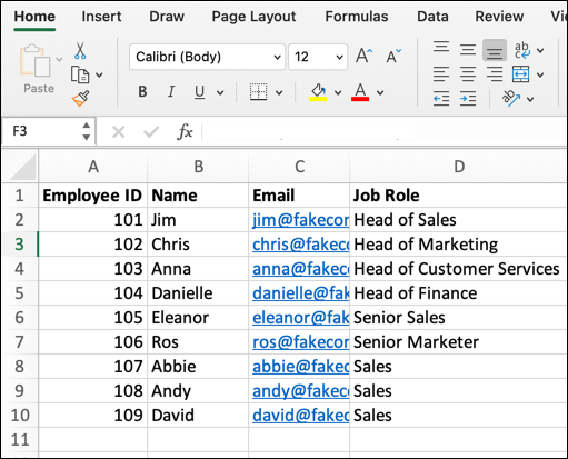
A dataset, such as this one, can be used as a searchable directory in Excel using an XLOOKUP formula. A search value for this formula could contain any of the values above, from an ID number to an email address.
XLOOKUP can find a value (matching in full or the closest approximation) from a range of cells (or search array) and return it. To do this, a formula using XLOOKUP has a number of arguments that need to be used to create the query.
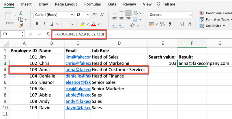
These include lookup, lookup_array, return_array, not_found (optional), match_mode (optional), and search_mode (optional). To create an XLOOKUP formula requires the following structure:
=XLOOKUP(lookup, lookup_array, return_array, not_found, match_mode, search_mode)
Required arguments (lookup, lookup_array, return_array)
In this example, lookup refers to the search value we’re looking for. For instance, if we’re looking for an ID number, we’d use the value itself (eg. 101) or a cell reference containing that value (eg. E3).
To find those values, we need to identify the cell ranges for the lookup_array and return_array. In this instance, the lookup_array is the column or row that contains the lookup value (eg. A2:A10 for ID numbers in column A).
The return_array is the individual column or row that contains the data that you want to return. For instance, if we’re searching for ID numbers, but want to return the employee name instead, we’d require the correct cell range containing those names (eg. B2:B10 for employee names in column B).
Optional arguments (not_found, match_mode, search_mode)
If you’d like to return a custom value when no results are matching, you’ll need to add a not_found argument. This could be a number, text string (in quotation marks), boolean value (TRUE or FALSE) or a cell reference (eg. 1, “not found”, or G1). If you don’t supply this, Excel will return an #N/A error for non-matching values.
XLOOKUP will, by default, search for exact matches to the lookup value. If you want to change this, you can supply the optional match_mode argument in your XLOOKUP formula. This is a numerical value, with 0 used for exact matches, -1 used for an exact match (or the next value below it), 1 for an exact match (or the next value above it), and 2 for wildcard values.
If you choose to use 2 for match_mode, you can use wildcard operators such as an asterisk (*), question mark (?) or tilde (~) with lookup values. Excel will return the first available match to the lookup value as a result.
Finally, you can determine the search order for values returned using the search_mode argument. XLOOKUP will immediately match the first value by default (the 1 value for search_mode, if you want or need to specify it), or you can reverse this to use the last matching value with -1.
You can also use binary searches in ascending order with 2 or descending order with -2. A binary search is essentially a fast type of recursive search using an ordered dataset, so you’ll need to make sure you’ve sorted your lookup_array and return_array data before using a search like this.
3. Things to consider before using the XLOOKUP function in Excel
The XLOOKUP function has significant improvements over earlier lookup functions, but there are a few things you’ll need to consider before you use it. These include:
- Unlike VLOOKUP or HLOOKUP, XLOOKUP is capable of using data both horizontally (in rows) or vertically (in columns).
- XLOOKUP can return a single result or multiple results, depending on the formula used. For a query like this, you’d probably need to use nested XLOOKUP functions in a single formula.
- If XLOOKUP can’t find a matching result and you want to see a custom error message, you’ll need to use the not_found argument (using numbers, text strings, boolean values, or cell references). Otherwise, Excel will return an #N/A error.
- While a different range can be used for the return_array argument value, it must be the same size (the same number of cells) as the lookup_array. If it isn’t, Excel will return a #VALUE error.
- XLOOKUP can be used to return values between different Excel spreadsheets, but both spreadsheets must be open for it to work. Otherwise, Excel will return a #REF! error.
- XLOOKUP returns a cell reference as the result, rather than the value. For example, if the lookup value of cell A2 is the number 4, then XLOOKUP will technically return A2, rather than 4 (although you’ll only see 4). This is a technical point that shouldn’t impact on (or be useful for) most XLOOKUP queries, but could prove useful for more complex searches.
- Nested formulas (containing multiple XLOOKUP functions) are possible, acting as a replacement for INDEX and MATCH combinations in complex lookup queries. These are performed in step (so if X = 1 and Y = 2, return Z). You can also use XLOOKUP with other functions (such as SUM or SUMIF).
- If you’re trying to use XLOOKUP in a version of Excel that doesn’t support it, you’ll see a #NAME error returned. You’ll need to switch to a supported version, such as the latest Microsoft 365 release, or by using Excel Online.
4. How to use XLOOKUP in Excel: A step-by-step guide
If you want to create a formula using the XLOOKUP function in Excel, you’ll need to follow these steps.
Step 1: Select an empty cell
To insert an XLOOKUP function in a new formula, start by opening an Excel spreadsheet containing your dataset and selecting an empty cell. Alternatively, open a new spreadsheet, leaving the spreadsheet containing your data minimized in another window.
Once the cell is selected, press the formula bar on the ribbon bar to begin to edit it.

The cell is active and ready for editing when the blinking cursor is visible on the ribbon bar. If this is the case, you’re ready to begin inserting a new XLOOKUP formula.
Step 2: Determine the search (lookup) criteria
As we explained above, a new formula using the XLOOKUP function has specific syntax and structure that needs to be followed. The first step is to begin to type the formula. To do this, type =XLOOKUP( in the ribbon bar.

The next step is to insert your lookup criteria. This is the data you’re looking to search for. While XLOOKUP supports numbers and text strings, most users will want to specify a cell reference (such as A2). This will allow you to change the search criteria (and thus the results) at will without changing the XLOOKUP formula directly.
For instance, using our employee list example, =XLOOKUP(E3 would use the value in cell E3 as the lookup value. In this instance, cell E3 contains the value 103, matching an ID number for an employee.
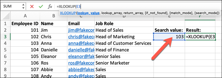
XLOOKUP will attempt to find the exact match by default. To change this, be sure to add an optional match_mode argument later (see step 5 below).
Step 3: Determine the dataset using lookup_array and return_array
Once you’ve inserted the lookup value (your search value, or a cell reference containing it), you’ll need to identify your lookup_array and return_array cell ranges.
The lookup_array is the row or column that is likely to contain your search query (or nearest approximate result). The return_array is the row or column that you’d like to see returned as a result.
This could be a cell in another column on the same line (matching ID numbers to job roles in our example employee spreadsheet, for instance).
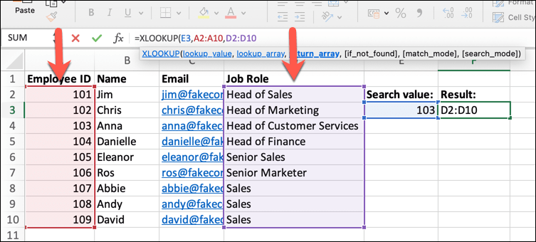
For our example, using =XLOOKUP(E3,A2:A10,D2:D10 means that the lookup_array used is the vertical cell range A2:A10, while the return_array is the vertical cell range D2:D10.
At this point, if you’re not interested in adding a custom error message, using a different search type (eg. approximate or wildcard matches), or changing the search value order, you can close your formula with a closing parenthesis. Otherwise, continue to add to your formula with optional arguments by following the steps below.
Step 4 (Optional): Add a custom error message using not_found
If you’re trying to find an exact match for your lookup value, but it can’t be found in your lookup_array range, Excel returns an #N/A error response. To overcome this, you’ll need to add an optional not_found argument to your XLOOKUP formula.
A not_found argument can be a numerical value (such as 1), a text string in quotation marks (such as “not found”), a boolean value (TRUE or FALSE), or a cell reference (such as A2).
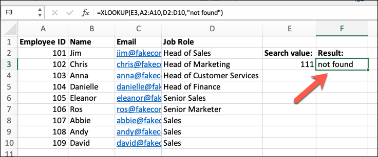
For instance, =XLOOKUP(E3,A2:A10,D2:D10,”not found”, would ensure that Excel returned a not found message if an exact match to the value in E3 can’t be found. As the ID numbers in the A2 to A10 cell range from 101 to 109, and the lookup value in cell E3 is 110, Excel returns not found as a consequence.
Because each argument is considered sequentially, you’ll need to add a custom not_found argument if you plan on adding further match_mode and search_mode arguments below to your formula.
Step 5 (Optional): Set exact, approximate, or wildcard search matches using match_mode
While XLOOKUP is designed to search for exact matches by default, this can be changed by adding an optional match_mode argument value to your formula.
There are four possible values: 0 for an exact match (the default value, if it isn’t added), –1 for an exact match or the next value below it, 1 for an exact match or the next value above it, or 2 for partial matches using asterisks, tildes, or question mark wildcards.
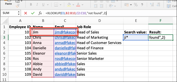
Using our example spreadsheet, the partial formula =XLOOKUP(E3,B2:B10,C2:C10,”not found”,2 would ensure that XLOOKUP supported a wildcard query. In this instance, XLOOKUP finds the nearest matching value to the wildcard query (ji*) in the lookup_array range B2:B10, then returns the matching value on the same row from the return_array range C2:C10 (an email address).
As a wildcard match, this would be the first, closest approximation. If you want to change the search order (for instance, using the last possible value, rather than the first), you’ll need to add a search_mode argument next.
Step 6 (Optional): Determine the value return order using search_mode
An optional search_mode argument is the final supported argument in an XLOOKUP formula. This changes the order in which XLOOKUP grabs a matching result. By default, Excel will try to match the first possible value.
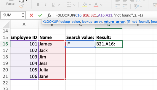
For instance, in a simple wildcard query where J* is the lookup value, an array containing the names James, Jack, Jim, Jess, Julia, and Jane would mean that 101 is the value typically returned, as James is the first value in a query where all values potentially match.
If you wanted to change this behavior to find the last possible value instead, you’d need to change the search_mode argument.
There are four possible values for a search_mode argument: 1 searches for the first possible value (this is the default option) while -1 reverses this to search for the last possible value. Alternatively, you can conduct a binary search in ascending order with 2 or reversed binary search in descending order with -2.
Binary searches can be quicker, reducing the number of searches through a data array to find the correct value (and thus reducing the overall memory impact of the query, especially with larger datasets), but you’ll need to sort your data first before you use it.
Most users will probably want to stick with 1 or -1 for search_mode, but if you’re working with a large amount of data, 2 or -2 will reduce the impact.
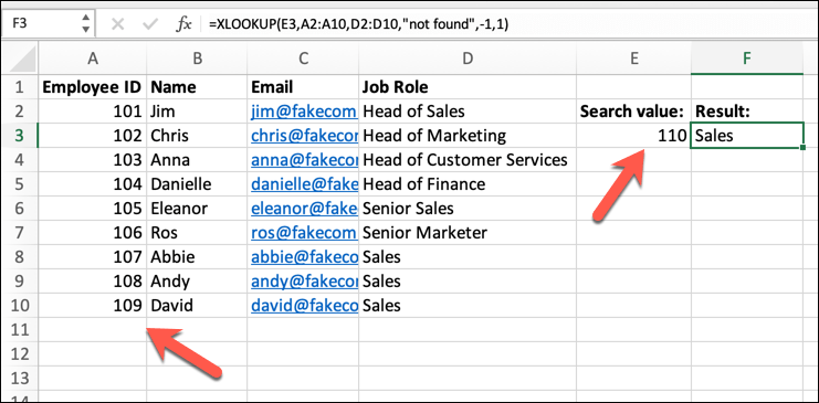
For instance, in the formula =XLOOKUP(E3,A2:A10,D2:D10,”not found”,-1,1), Excel finds the exact match or next and smallest value matching the lookup value in cell E2 and returns it. With search_mode set as 1, Excel will search in ascending order, returning the first matching value in the range.
In this instance, with the value in E2 set as 110, and with no values offering an exact match, the next and smallest result is ID number 109.
If you’ve used all optional arguments in your XLOOKUP criteria, make sure to close your formula with a closing parenthesis and press enter (or click on another empty cell) to see the result of your XLOOKUP query.
Final thoughts
If you’re looking to search through complex Excel spreadsheets, lookup functions like XLOOKUP offer the best way to do it. Data analysis is all about manipulating data to find the answers you’re looking for—XLOOKUP is one of many essential Excel formulas that data analysts need to have in their repertoire to do just that.
If you’re new to data analysis and you’re trying to build your skillset a little further, you can try out CareerFoundry’s free data analytics short course, with five daily lessons to help you see whether it’s the right career track for you. For those curious to learn more, we’ve got a number of useful articles you can take a look at next, including:
