The VLOOKUP function in Microsoft Excel is a search tool that allows you to look up data in a table, where each row is an entry and each column holds different types of data. We’ll explain how to use the VLOOKUP function, step-by-step, in this tutorial.
The VLOOKUP function is one of several lookup functions included in Microsoft Excel that allows you to locate and return approximate or exact matches from data organized in a table format, depending on the arguments you use. VLOOKUP works with data stored vertically, with each column in a data set having a different purpose.
While newer lookup functions like XLOOKUP offer more functionality, VLOOKUP is tried-and-tested, with availability for older Excel versions. As long as you avoid some of its limitations, VLOOKUP remains one of the easiest, most powerful search tools for Excel data analysts.
In this article, we’ll explain:
- What is the VLOOKUP function and how does it work?
- How does the VLOOKUP function work in Microsoft Excel?
- Things to consider before using the VLOOKUP function in Excel
- How to use VLOOKUP in an Excel formula: A step-by-step guide
Are you finding it difficult to use the VLOOKUP function in your spreadsheet to search through your data? We’ll explain everything you need to know in this guide.
1. What is the VLOOKUP function and how does it work?
There are a number of built-in search tools for Excel users. If you wanted to visually emphasize certain data, you could add conditional formatting rules to your spreadsheet. If you want to quickly find a number or a text string, you could use “find” and “select.”
These are fairly basic tools for searching through your spreadsheet data, however. If you want to create searches that interact with your data directly and return results you could use elsewhere, you’d need to use a lookup formula. Several of these exist, but one of the easiest to use is VLOOKUP.
VLOOKUP, or vertical lookup, allows you to look up data that’s sorted vertically, in tables where each row is a result, with various (related) information spread across different columns. A class result list, for instance, may have student names, ID numbers, and exam results in each column, where each student is on a single row.
There are some limitations to using VLOOKUP that can be problematic, however. You can only search for data to the right of your lookup value, so you’ll always need to look for data that’s in a column to the left. If your data is sorted horizontally, you’ll need to use another function like HLOOKUP or XLOOKUP instead.
2. How does the VLOOKUP function work in Microsoft Excel?
The VLOOKUP function is a lookup function designed to help you find data organized vertically in a table, where a single row may contain related data across several columns.
Let’s explain this using an example scenario. An example Excel spreadsheet contains a student class list, with student ID numbers, names, email addresses, and their most recent exam results.
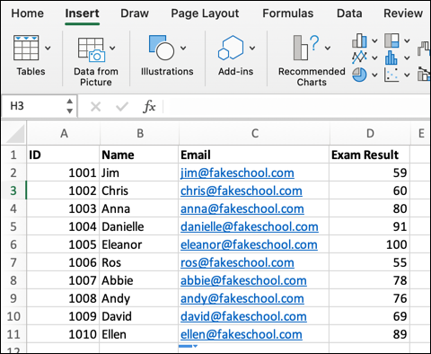
The data is organized in a table, where each row represents a student, and each column contains information about that student. To look up specific information about a student, you’d need VLOOKUP to find a matching value from any of the columns.
For instance, matching ID number 101 would ensure that, in this scenario, VLOOKUP can find any of the information to the right of that value, including their email address and exam result.
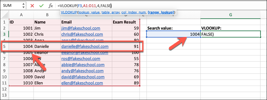
VLOOKUP has several arguments that can be used. These include value, table, col_index_num and the optional range_lookup. To create a VLOOKUP formula using these arguments requires this structure:
=VLOOKUP(value, table, col_index_num,range_lookup).
In this example, value is the search value we’re trying to find in our table. We could, for instance, be looking for a matching student ID number (eg. 1010). If we wanted to create an easily-edited search box, we could refer to a cell reference that contained this value instead (eg. F3).
To do this, you need to identify the table containing your data. This is typically a cell range, such as A2:D11. Once VLOOKUP finds the row containing your lookup value criteria, you’ll then need to identify the data from that row that you’d like it to return.
To do this, you’ll need to pinpoint the column containing the result that you want to return. Just like you might identify a cell range by using the row number and column letter, the VLOOKUP formula already knows the row, based on the matching search value.
It now needs the right column, which requires a col_index_num value as a number. Starting with the number 1 for the first column in your table, you’ll need to identify the right column (for instance, 3 for column C).
Finally, you’ll need to identify whether you want VLOOKUP to return an exact match (the first matching result in an organized and sorted table) or return approximate matches instead. To set this, you’ll need to add a range_lookup value to your formula.
This is a boolean choice, with only TRUE or 1 (for approximate matches) or FALSE or 0 (for exact matches) available. If you don’t provide a range_lookup value, Excel will use TRUE and return an approximate match instead, which may not be appropriate for a search like this.
If you’re using a lookup value with wildcards, you’ll need to set the range_lookup to TRUE (for exact matches) to return the correct value.
3. Things to consider before using the VLOOKUP function in Excel
There are a number of things you’ll need to consider before you decide to use a VLOOKUP function in Excel. These include:
- VLOOKUP looks for data to the right of any lookup value. Trying to find data to the left will result in an error. You can get around this by using the INDEX and MATCH functions or by using the newer XLOOKUP function.
- VLOOKUP is a vertical lookup function. That means that your data needs to be organized in a table where each row has different (but related) forms of data in each column. If you want to search for data in other formats, use HLOOKUP, INDEX and MATCH, or XLOOKUP instead.
- By default, VLOOKUP returns the first approximate match to the lookup value. You can change this by setting a range_lookup argument in your formula, where TRUE returns approximate matches while FALSE returns exact matches. You can use numbers (0 or 1) or text (FALSE or TRUE).
- Exact matches in VLOOKUP formulas actually refer to the first exact match in the table. This might prove problematic for data tables where the lookup value has several matching results, so sort your data accordingly.
- If you’re trying to search for an approximate match, your data will need to be manually sorted in ascending order for the results to be correct.
- Be careful inserting new columns into your data table, as this can break col_index_num values in your existing VLOOKUP formulas.
- Wildcards can be used for VLOOKUP lookup values using asterisks or question marks. You’ll need to use an ampersand to concatenate the lookup value with the wildcard within your VLOOKUP formula (eg. VLOOKUP(value&“*”, table, col_index_num, range_lookup) for this to work correctly.
- VLOOKUP isn’t designed to look for case-sensitive text and will return the first exact or approximate matching value, regardless of the text case used.
4. How to use VLOOKUP in an Excel formula: A step-by-step guide
To begin using the XLOOKUP function in Excel, you’ll need to create a formula using it—here’s how.
Step 1: Select an empty cell
To insert a new VLOOKUP formula, you’ll need to first open the Excel spreadsheet containing your data. Alternatively, open a new spreadsheet alongside the existing spreadsheet that contains your data. You’ll need to keep the other spreadsheet minimized to use that data, otherwise Excel will return an error.
In the new (or existing) sheet, select an empty cell, then press the formula bar at the top of your window, situated at the bottom of the ribbon bar.
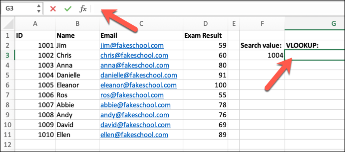
The cell is ready for you to edit once the blinking cursor is visible in the formula bar itself.
Step 2: Determine the lookup value
If you’re inserting a new VLOOKUP formula, you’ll need to use the correct structure (as we explained above). The first step is to insert a new formula by typing =VLOOKUP( in the formula bar.
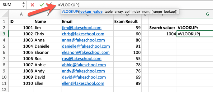
The first stage of a VLOOKUP formula is to add your lookup value—the value you’re searching for. This could be a number, text string, or a cell reference for a cell that contains your search value (eg. A3). If you choose a cell reference, you can change your search value later without changing the formula directly.
To give an example, =VLOOKUP(100 would use the number 100 as the lookup value. Alternatively, =VLOOKUP(F3 would use the value in cell F3 as the lookup value. VLOOKUP can only look for data to the right of matching values, so bear this in mind before you insert your lookup value.
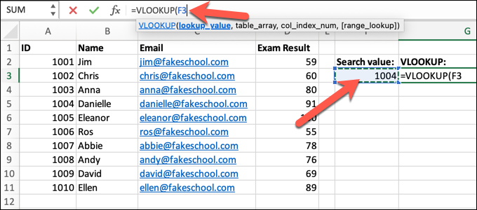
You can also use a wildcard (an asterisk or question mark) for partial matches. For instance, =VLOOKUP(100 & “*”, will search for the nearest partial match to the value 100. This uses concatenation (using an ampersand, rather than the CONCATENATE function) to link the lookup value to the wildcard.
Similarly, you could use =VLOOKUP(D3 & “*”, to use the value in cell D3 with a wildcard to search for a partial match instead.
By default, VLOOKUP will search for approximate matches. If you want to look for an exact match, you’ll need to add the optional range_lookup value at the end of your formula. You’ll need to add a range_lookup value if you want to use a wildcard.
Step 3: Identify the table containing your data
If you’re using VLOOKUP, your data set needs to be arranged vertically in a table, with each column representing different data. Once you’ve added your lookup value to your new VLOOKUP formula, you’ll need to identify the cell range containing your data.
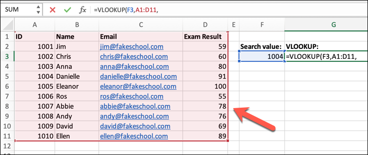
To do this, add the range to your open VLOOKUP formula. For instance, the formula VLOOKUP(100,A1:D11, would instruct Excel to search for the lookup value 100 in a cell range between A1 and D11.
Each column in that range (from A to D) holds different information. Once Excel identifies the matching value (or nearest match), VLOOKUP can then return any of the data on that row (from cells in columns A to D).
Step 4: Add the column index (col_index_num) value
With your data table and lookup value identified, the next step is to pick out the data you wish for VLOOKUP to return. To do this, you’ll need to add a col_index_num (column index) value to your formula.
Rather than using letter identifiers for each column, VLOOKUP uses numbers. Starting with the number 1, each col_index_num value increases sequentially for the columns in the data range you identified. For example, if your data table ranges from A1 to D11, column A is 1, B is 2, etc.
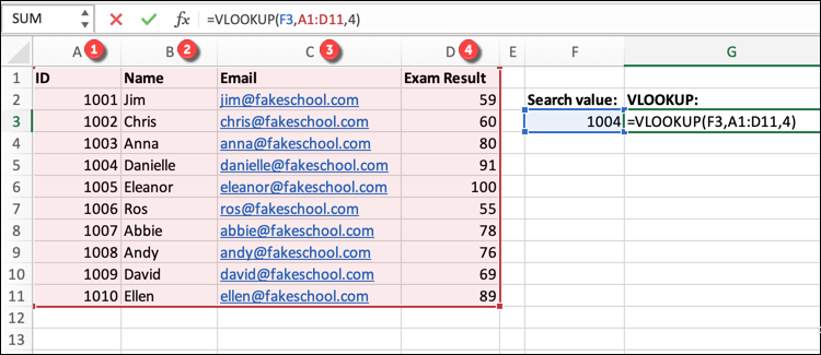
However, you must choose a col_index_num value that is to the right of the lookup value. This is a limitation of VLOOKUP that only a replacement formula like XLOOKUP can resolve. To add your col_index_num value, simply add the number that matches the column to your formula.
For instance, =VLOOKUP(100,A1:D11,2 would find the matching row with value 100 from a table in cells A1 to D11, returning the matching value in the same row from column 2 which, in this instance, would equate to column B.
At this point, you can close your formula using a closing parenthesis if you’re happy to search for an approximate match. To do this, add a ), then press enter or select an empty cell to view the result.
If you want to change this to search for an exact match, you’ll need to add a further range_lookup value, as explained below.
Step 5 (Optional): Set exact or approximate matches using range_lookup
The optional range_lookup argument allows you to set whether VLOOKUP searches for an exact or approximate match. This is a true boolean choice, with only TRUE or 1 (for approximate matches) or FALSE or 0 (for exact matches) as the available options.
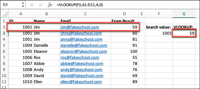
While adding a range_lookup value is optional, most users will probably want to do so. This is because VLOOKUP, by default, searches for an approximate match. If you have several values in your data set that are near-matches, this could result in the wrong data being returned.
For example, =VLOOKUP(100,A1:D11,2,FALSE) would find the exact match for value 100 from column 2 (column B) in a data table from cell ranges A1 to D11. Once you’ve closed your formula with a closing parenthesis, press the enter key or select an empty cell to view the result.
If you wanted to find the approximate match, you could end with a closing parenthesis after the col_index_num value, or use the formula =VLOOKUP(100,A1:D11,2,TRUE) instead.
You can also use numbers as range_lookup values, where 1 equals TRUE and 0 equals FALSE. For instance, the formula =VLOOKUP(100,A1:D11,2,1) would work for approximate matches instead.
Final thoughts
When you’re trying to quickly search for data in an Excel spreadsheet, lookup functions like VLOOKUP are perfect for the job. That said, if you’re a Microsoft 365 subscriber, the newer XLOOKUP function offers speed and functionality enhancements that are absolutely worth considering for future spreadsheets.
New data analysts don’t need to worry about figuring things out on their own, because our free five-day short course will help to bring you up to speed with the kind of skills you’ll need to learn.
Want more Excel tutorials? Check out the following:
