The SUMIF function in Microsoft Excel allows you to calculate the combined values of different cells, based on a specific criteria. In this tutorial, we’ll explain, step-by-step, how to use the SUMIF function.
If you’re using Excel for data analysis, then it’s quite likely that you’re already using the SUM function to combine your data. The word sum simply means total, but if you’re dealing with a large amount of data, it’s probable that you don’t want the full total from a range of cells, but rather a selective total value instead.
You can learn more Excel analysis skills with our free 5-day data short course.
Thanks to the SUMIF function, this is entirely possible. In this guide, we’ll explain:
- What is the SUMIF function and what is it used for?
- How does the SUMIF function work in Microsoft Excel?
- Things to consider before using SUMIF in Excel
- How to use SUMIF in an Excel formula: A step-by-step guide
Are you looking to get to grips with the SUMIF function yourself? To help you, let’s explore how it works and how to use it.
1. What is the SUMIF function and what is it used for?
As we’ve mentioned, to calculate the sum (total) of a range of cells, you’d typically use the SUM function in Microsoft Excel.
However, SUM is a very basic function that doesn’t allow the end user to determine which cells it should choose to include in the formula: it simply includes them all.
This makes SUM a less useful function for complex data analysis. To get around this, you can use SUMIF instead. SUMIF allows you to use a logical statement (in this case, an IF statement) to help Excel determine what cells it should consider before it calculates the total value.
We’ll give you an example. If you have a list of students collecting money, and you’re trying to determine the total based on what “team” they belong to (say, red or blue), you could use SUMIF, where the function would determine the total value of sponsorships if the students are a member of, say, the red team.
The limitations of an IF statement in this way means that, if you use the SUMIF function, you can only have a single criteria (eg. cell range contains “male”).
If you require additional criteria for your logical statement, you would need to use an alternative function like SUMIFS instead, which allows you to combine IF with AND operators in a single formula.
2. How does the SUMIF function work in Microsoft Excel?
The SUMIF function is an extension of the existing SUM and, like the original, can be pretty simple to use.
Like SUM, SUMIF works by calculating the total of a range of cells together but, unlike SUM, it does this by using criteria to determine which cells to include, rather than including them all.
The criteria used to determine whether a cell can be included in the formula can be a number (eg. whether the cells contain the number 12), a text string (eg. cells containing the word “yes”), and contain a mathematical operator (eg. values greater than 12).
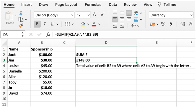
A formula using the SUMIF function has three arguments: range, criteria, and sum_range (where sum_range is optional). Creating a formula using the SUMIF function is simple, and relies on a simple structure, which is as follows:
=SUMIF(range, criteria,sum_range)
In this example, range refers to the cell range you wish to use as part of your criteria check (eg. A2:C1). The criteria argument, as the name suggests, refers to your single IF criteria (eg. checking for a text string containing the word “today”).
The optional sum_range argument allows you to determine a second cell range to use for your SUMIF calculation. This can be useful if you want to use the initial range argument for your logical operation, but want to know the total from a different set of cells (eg. if X equals Y sum Z).
While you could also use pivot tables to calculate the sum of a range of cells using criteria, the SUMIF function is a quicker and cleaner method to get the job done.
3. Things to consider before using SUMIF in Excel
The SUMIF function has few limitations, but they do exist, so you’ll need to watch out for them. These include:
- Without a sum_range argument, the cell range referenced in the initial range argument will also be used for the SUMIF calculation.
- The use of an ampersand (&) allows for basic concatenation within a SUMIF formula, allowing you to use data from other cells as part of a SUMIF criteria argument. For instance, =SUMIF(A2:D1, “<”&A9) would look for cells in the A2 to D1 range that are less than the value of the cell A9.
- Concatenation using an ampersand can also be used with other functions, such as the DATE function, to allow for more complex criteria.
- If your criteria uses a text string, you can use wildcards to search for partial matches (such as ? to search for characters by length or * for characters in sequence). If you need to search for these special characters (rather than use them as part of your criteria), place a tilde symbol in front of them (eg. ~*).
- Text strings, used as part of the criteria argument, can be a maximum of 255 characters long. Longer strings will return a #VALUE! error message.
4. How to use SUMIF in an Excel formula: A step-by-step guide
If you want to use the SUMIF function in an Excel workbook, you’ll need to follow these steps.
Step 1: Select an empty cell
You can start by opening an Excel spreadsheet and selecting an empty cell. With the cell selected, press the formula bar on the ribbon bar to focus on it.
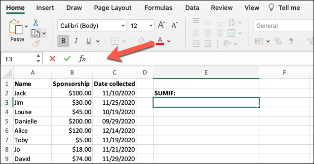
With your blinking cursor active in the formula bar, you can begin to create your SUMIF formula.
Step 2: Determine the initial cell range
With the formula bar active, you’ll need to begin to write your SUMIF formula using the structure and syntax described above. Start by typing =SUMIF( in the ribbon bar.
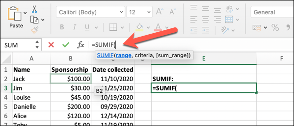
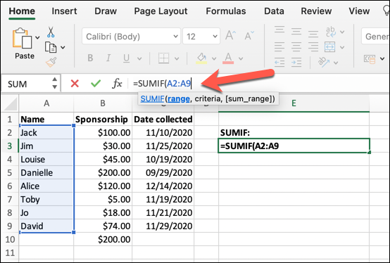
You’ll then need to select the initial cell range. If you’re not using the sum_range criteria at the end of your formula, this will contain the data that the SUMIF function will calculate to determine the total. Otherwise, this data will be used for testing against your criteria only.
To do this, type your cell range by using the first and last cell in the range or by selecting the cells using your mouse or touchpad. For instance, =SUMIF(A2:A9, will use a cell range between A2 and A9.
Step 3: Determine the SUMIF criteria
With the initial range selected, you’ll need to determine the SUMIF criteria. This is the logical IF operatortest that the formula will use to pick out which cells will be counted and which cells will be ignored.
You can use numbers, text strings, mathematical operators, wildcards and other cell references as part of your criteria.
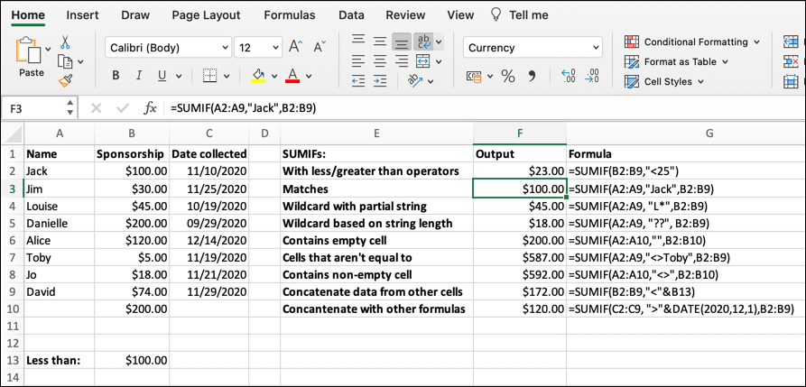
Examples of different SUMIF criteria include:
- Using less or greater than operators: =SUMIF(B2:B9, “<25”)
- Matches a text string: =SUMIF(A2:A9, “L*“,B2:B9)
- Using a wildcard to match a partial string: =SUMIF(A2:A9, “to*”)
- Using a wildcard to find cells that have a certain character length, based on the number of question marks used: =SUMIF(A2:A9, “??”, B2:B9)
- All cells within range that are empty: =SUMIF(A2:A10,”“,B2:B10)
- Cells that aren’t equal to the criteria: =SUMIF(A2:A9,”<>Toby”,B2:B9)
- All cells within range that aren’t empty: =SUMIF(A2:A10,”<>“,B2:B10)
- Uses concatenation to add data from other cells: =SUMIF(B2:B9,”<“&B13)
- Uses concatenation to correctly use dates: =SUMIF(C2:C9, “>“&DATE(2020,12,1),B2:B9)
These examples can be adapted to suit your own needs and aren’t an exhaustive list. If you intend on using your initial cell range as part of your calculation, you’ll need to close the formula with a closing parenthesesto see the output result, such as =SUMIF(A2:A9,”<25”>).
Step 4 (Optional): Determine your sum_range criteria
The final argument of a SUMIF formula (sum_range) is optional, and can be used to create more complex logical tests.
If you wanted to test one cell range before calculating the SUM of the second, you’ll need to add your sum_range criteria before closing the formula.
As with the initial range criteria, provide the first and lastless cells in your range before closing the formula with a closing parentheses.
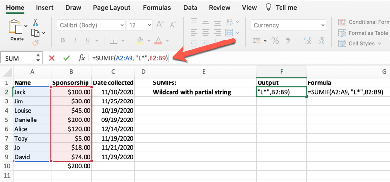
For example, =SUMIF(A2:A9, “L*“,B2:B9) will match cells between A2 and A9 to see if they contain text strings beginning with the letter L. If they do, the matching numbers in cells in B2 to B9 will be calculated using SUM.
Excel will return a #VALUE! or similar error message if your cell ranges or criteria are incorrect.
Final thoughts
Functions like SUMIF are useful in quickly extrapolating data from an Excel spreadsheet.
While alternatives like SUMIFS and pivot tables could help you with more complex analysis, SUMIF should prove useful for smaller data sets. It’s also one of several Excel formulas considered essential for data analysts to regularly use—like the AVERAGE function, XLOOKUP, and COUNTIFS, to name just a few!
Data analytics can seem like a difficult subject to crack, but if you’re a beginner, you can hit the ground running with a free five-day short course. If you’d like to learn more about the tools and techniques used by data analysts, check out the following:
