The INDIRECT function in Excel is used to create a reference specified by a text string. It enables us to create references from cell values.
This function is one of the lookup and reference functions in Excel. It is most used for building dynamic references for calculations and chart ranges.
The INDIRECT function defaults to an A1 style reference, but has the option to switch to a R1C1 reference style.
In this tutorial, we’ll show you how to use the INDIRECT function to reference other sheets, tables, and named ranges from cell values. We will also demonstrate both the A1 and R1C1 reference styles.
We’ll cover:
- What is the INDIRECT function and why use it?
- How to use the INDIRECT function
- Things to consider when using the INDIRECT function
- Use the INDIRECT function to reference other sheets
- Reference tables with INDIRECT
- INDIRECT function and R1C1 references
So, let’s dive into the INDIRECT function. You can use this worksheet to practice.
1. What is the INDIRECT function and why use it?
The INDIRECT function is very useful for building dynamic references for our reports and other analysis in Excel.
It enables us to use cell values and text strings for formula references instead of writing the reference directly into a formula such as a COUNTIFS or a VLOOKUP.
The INDIRECT function requires only two arguments.
=INDIRECT(ref_text, [a1])
Ref text: A text string or reference to a cell that can be used as a range reference.
a1: A logical value to specify whether you want to use A1 or R1C1 style references. This argument is optional. Omit the argument or enter True to use A1 style. Enter False to specify the use of R1C1 style.
2. How to use the INDIRECT function
You can download the Excel workbook to follow along with the examples in this tutorial.
In this first example, we will see a basic use of the INDIRECT function to understand the principles behind its use.
In cell B2 the following formula has been entered.
=INDIRECT(C2)
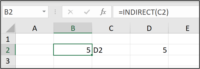
This formula converts the text value in cell C2 into a reference. So the INDIRECT function returns the value from cell D2. The second argument is omitted in this example, so an A1 reference style is used.
This is a very basic example that is not very practical, but it helps to understand how the INDIRECT function works.
Let’s see an example of the INDIRECT function with named ranges.
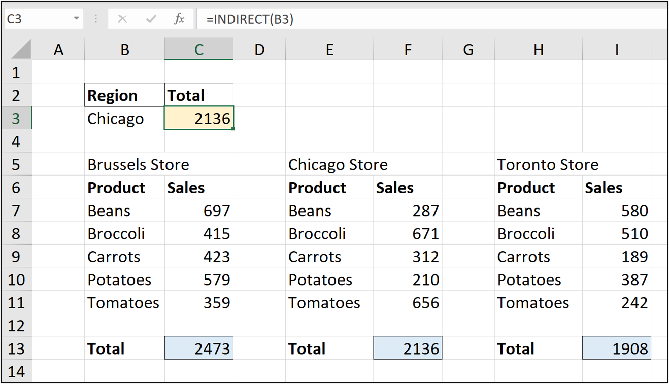
In this example, cells C13, F13 and I13 have been named Brussels, Chicago, and Toronto. The following formula has been entered into cell C3. It indirectly references a named range using the value in cell B3. This value is selected from a drop-down list.
=INDIRECT(B3)
3. Things to consider when using the INDIRECT function
There are a few things to be aware of when using the INDIRECT function.
- Ensure that the reference exists. A #REF! Error is produced if the INDIRECT text does not match a reference. This could be a typo in the formula, or maybe in the name of a range, table, or sheet.
- The #REF! error is also shown if the INDIRECT function references another workbook, and that workbook is closed.
- The ampersand (&) is used to combine text and cell values to form a complete string that can be used as a reference.
- If a sheet name contains spaces, it should be enclosed in single quotes (‘) in the reference. For example, ‘New Jersey’!B2 would be the reference to cell B2 of a sheet named New Jersey.
4. Use the INDIRECT function to reference other sheets
One of the most common uses of the INDIRECT function is to reference other sheets using the value of a cell.
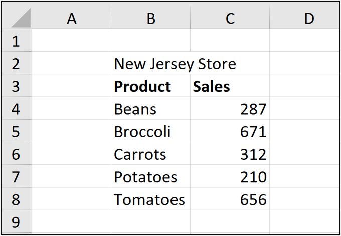
In this example, we have three worksheets named Brussels, New Jersey, and Toronto. The image shows the data in the New Jersey sheet. All three sheets are structured the same.
The following formula is used to sum the values from range C4:C8 on the sheet specified by the value in cell B3.
=SUM(INDIRECT(“’“&B3&”’!C4:C8”))
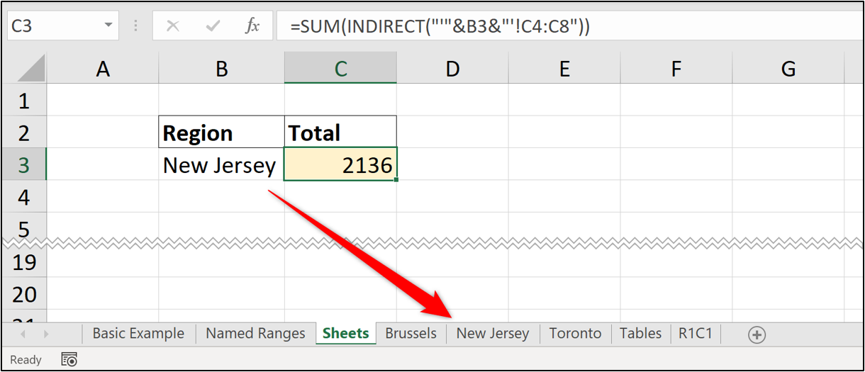
The ampersand is used to join the parts together into a complete reference. The first part is the single quote, the second part is the value from cell B3, and the final part is the closing single quote followed by the exclamation mark and range reference.
The single quotes are required because the sheet named New Jersey contains a space.
The INDIRECT function creates this reference for the SUM function to then use.
5. Reference tables with INDIRECT
The INDIRECT function provides a dynamic way of referring to a table. These tables can be on any sheet in the workbook and provide a cleaner method than referencing sheet names like the previous example.
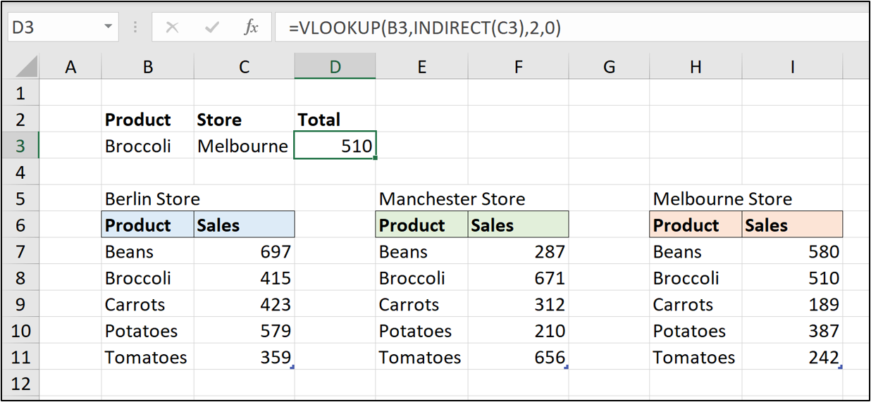
In this example, the tables are all on one sheet to show the formula more easily. A VLOOKUP function is used to return the value for a specified product (value in cell B3) from the table specified in cell C3.
The INDIRECT function is used to convert the text in cell C3 to a reference for the VLOOKUP function.
=VLOOKUP(B3,INDIRECT(C3),2,0)
6. INDIRECT function and R1C1 references
All of the examples so far have demonstrated INDIRECT with the A1 style reference, which is most common. Let’s now see an R1C1 style used.
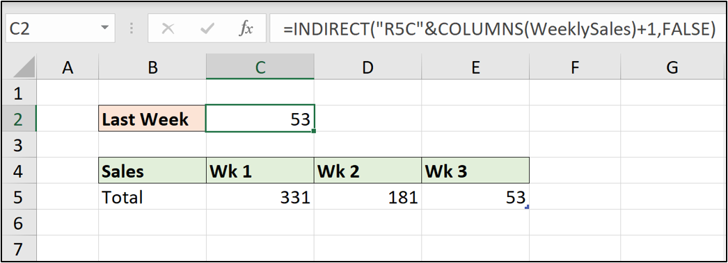
In this example, we want to return the value for the last week.
The data is formatted in a table named WeeklySales. In the INDIRECT function, the text “R5C” is joined with the result of the columns function +1.
This results in R5C5. There are 4 columns in the table, then + 1. So return the value from the fifth row and fifth column of the sheet. The FALSE specifies to use R1C1 referencing.
=INDIRECT(“R5C”&COLUMNS(WeeklySales)+1,FALSE)
This example is demonstrated for better understanding of the INDIRECT function, however it is not an efficient way of performing this task. The INDEX function provides a better method.
Final thoughts
Excel formulas are an extremely handy tool for anyone working with data—especially data analysts. For a hands-on introduction to the field of data analytics, try out this free five-day short course. And, for more Excel tutorials, check out the following:
