The IFERROR function in Excel is used to trap formula errors and return another value or run another formula in their place.
Formula errors happen. But not all errors are the same. Some of them are predicted and do not mean that the formula is wrong.
These errors need to be dealt with effectively as they can break subsequent formulas or features such as PivotTables.
In this tutorial, we’ll show you how to use the IFERROR function. We’ll also provide some examples of how IFERROR can be used to handle errors from different Excel formulas.
We’ll cover:
- What is the IFERROR function and why use it?
- How to use the IFERROR function (step-by-step)
- Things to bear in mind when using the IFERROR function
- IFERROR with VLOOKUP
- IFERROR with the FILTER function
So: What is the IFERROR function? Let’s find out.
1. What is the IFERROR function and why use it?
The IFERROR function was introduced in 2007. It’s used to check if a formula evaluates to an error, and if so, determines a different course of action to be taken.
This action is often to display a different value or run an alternative formula.
Formula errors, even if innocent mistakes, can cause problems further down the line. So if we’re aware of these occurrences, the IFERROR function provides us with an easy-to-use error handling tool.
The IFERROR function requires only two arguments.
=IFERROR(value, value_if_error)
Value: This is what is being checked for an error. It is usually a formula, but can also be a cell reference or a logical expression.
Value if error: The action that should be performed if an error is returned.
A small and simple function. Let’s see it in action.
2. How to use the IFERROR function (step-by-step)
In this example, an error has occurred when evaluating the following formula down column D.
=C2/B2
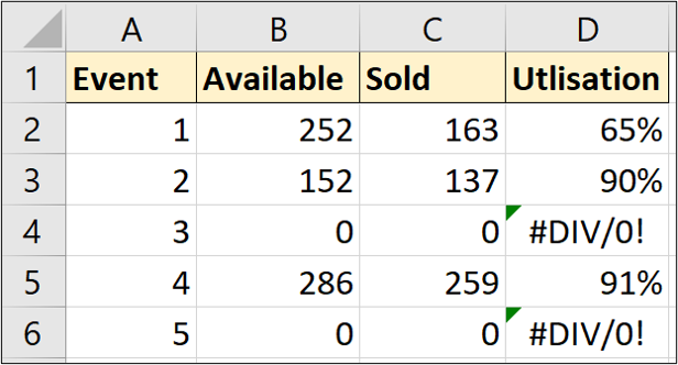
You cannot divide a value by zero, empty cells or text. And so an error is produced.
In an example such as this, the zero values are temporary, and soon there will be values in the “Available” column.
To prevent the error, the IFERROR function can be used. In this example, it checks the formula C2/B2 and returns 0 instead of an error.
=IFERROR(C2/B2,0)
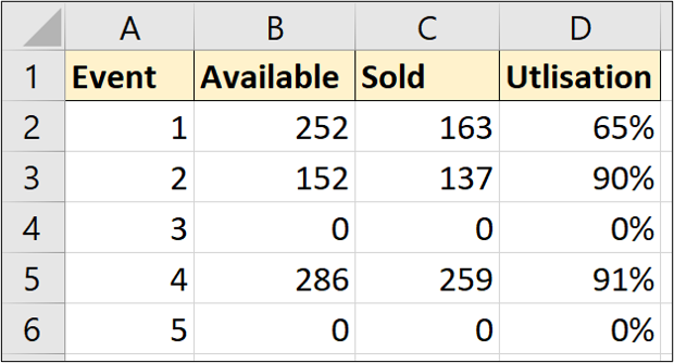
Simple and effective.
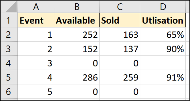
The IFERROR function can also be used to return a blank cell instead of an error message.
To do this, an empty string (“”) can be used for the value_if_error argument.
=IFERROR(C2/B2,””)
3. Things to bear in mind when using the IFERROR function
The most important thing to bear in mind when using the IFERROR function is to be sure that it’s not a real error caused by a formula.
IFERROR is incredibly helpful when it comes to trapping harmless errors, but should never be used to cover up real issues.
4. IFERROR with VLOOKUP
One of the most common uses of the IFERROR function is with lookup formulas such as VLOOKUP.
The VLOOKUP function returns the #N/A error message if it cannot return a value.
Now, this may be due to a mistake in the formula, but it is often because of some other reason.
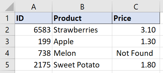
In this example, a VLOOKUP function is being used to return the price of the products from a table named “products”.
=VLOOKUP(A2,products,3,0)
An error has been generated when trying to return the price of “Melon.”
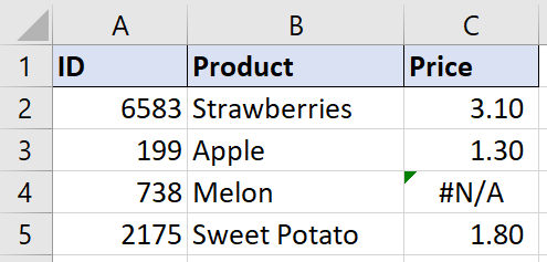
Instead of displaying the error, we can use the IFERROR function to display an alternative message such as “Not Found”.
=IFERROR(VLOOKUP(A2,products,3,0),”Not Found”)
IFERROR vs. IFNA
There is also a function named IFNA in Excel, which performs a very similar job to IFERROR.
The IFNA function was released in 2013 and traps the #N/A! Error only. It specifically targets the error generated in the VLOOKUP example.
The IFERROR function, however, can be used to trap any Excel formula error.
In the previous example, either function can be used for the job. However, it is more common to see IFERROR used as it’s been around since 2007.
If someone is using an Excel version prior to 2013, for example Excel 2010, then the IFNA approach is not compatible for them.
5. IFERROR with the FILTER function
Some recent lookup functions now have built-in error handling. These functions include XLOOKUP and FILTER.
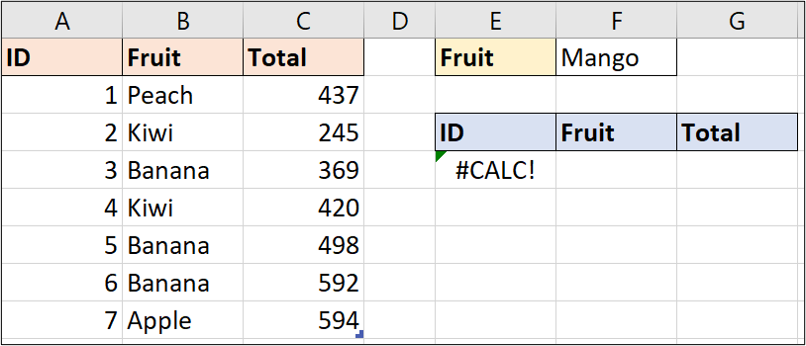
This FILTER function example filters the table to only show the sales for the fruit entered in cell F1. There are no sales of mango, so the #CALC! Error is shown.
=FILTER(fruitSales,fruitSales[Fruit]=F1)
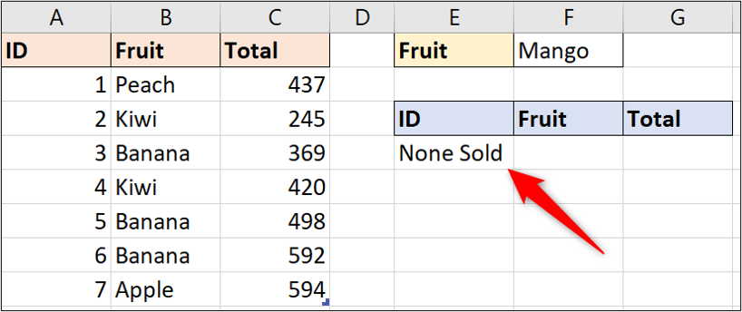
Now, the FILTER function has a third argument named if_empty, so that if no results are returned, an error is prevented and an alternative action is performed.
In this case, the text “None Sold” is displayed.
=FILTER(fruitSales,fruitSales[Fruit]=F1,”None Sold”)
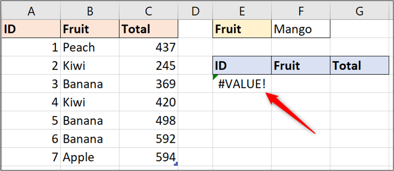
This is great! However, if we add to the formula with a SORT function to order the results descending by “Total”, as follows:
=SORT(FILTER(fruitSales,fruitSales[Fruit]=F1,”None Sold”),3,-1)
…the built-in error handler of FILTER can no longer help us and an error is produced.
So an IFERROR function can be added to display the text “None Sold” in this scenario.
=IFERROR(SORT(FILTER(fruitSales,fruitSales[Fruit]=F1),3,-1),”None Sold”)
With the involvement of IFERROR, the if_empty argument of FILTER is no longer needed. The IFERROR function can handle an error returned by any part of the formula.
So, IFERROR remains an important function,even with the vast improvements in modern Excel.
Final thoughts
Excel formulas are an extremely handy tool for anyone working with data—especially data analysts. For a hands-on introduction to the field of data analytics, try out this free five-day short course. And, for more Excel tutorials, check out the following:
