The IF function in Excel compares existing data in the spreadsheet against the value you set in the IF function’s Logical_test field. It then returns one of two values depending on whether the comparison was true or false.
The IF function is categorized as a Logical function, and is one of the most commonly-used functions in Microsoft Excel.
In this tutorial, we’ll show you how to use the IF function, as well as provide some real-world use cases.
We’ll cover:
- What is the IF function in Microsoft Excel?
- What is the IF function used for?
- How to use IF in Excel: A step-by-step tutorial
- Determining outcomes with IF
1. What is the IF function in Microsoft Excel?
Excel comes packed with a long list of Logical functions. All of Excel’s Logical functions perform actions based on the results of the specific function’s test. The IF function returns a result by comparing data that exists against a value you set. Here’s how the IF function looks:
=IF(Logical_test,Value_if_true,Value_if_false)
In other words, the Logical_test value checks if a condition is met and then returns a predetermined true or false value.
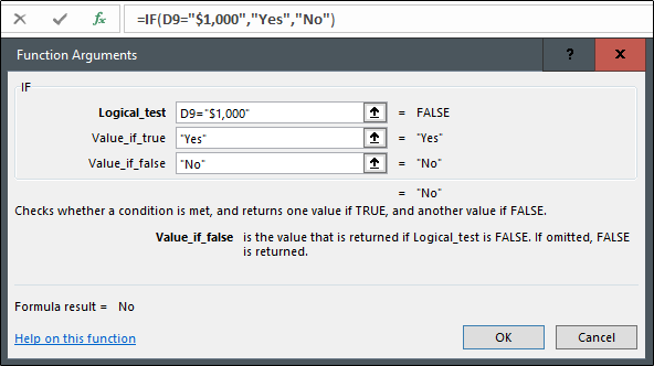
So in this example, we have:
=IF(D9=”$1,000”,”Yes”,”No”)
In human language, this means that if cell D9 is equal to $1,000, then return “Yes.” If not, return “No.”
While this example is certainly an oversimplification of what the IF function can be used for, it is the basic concept of how the function works.
2. What is the IF function used for?
The IF function is one of the most widely-used and popular functions in Microsoft Excel, largely due to its ability to be used in a wide number of scenarios. Here are a few situational examples of when using the IF function would be ideal.
Business
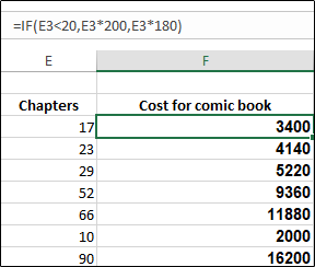
There are numerous scenarios in which the IF function would come in handy in business. Let’s say you work for a publishing company and you buy and sell rights for comic books. If a comic book has 20 chapters or more, your company will purchase the rights for that comic book for $180 per chapter. If it’s less than 20 chapters, your company will pay $200 per chapter. If you have a long list of comic books you’re interested in buying rights for, you can use the IF function to quickly determine how much you’ll need to pay to own the rights for the comic book based on the number of chapters in the comic.
In this scenario, we would use this formula:
=IF(E3<20,E3*200,E3*180)
So, if the number of chapters in cell E3 is less than 20, multiply the number in E3 by $200. Otherwise, multiply the number by $180.
Education
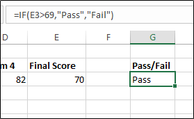
Without a doubt, the most common true/false scenario in education is the question of passing or failing a class. If the minimum score required to pass a class is 70, you can use the IF function to produce a pass or fail result based on the final score of the student.
The formula we would use in this situation would look something like:
=IF(E3>69,”Pass”,”Fail”)
So, if the student’s final score in cell E3 is greater than 69, return “Pass.” If it’s 69 or below, return “Fail.”
Personal
You’re going on a vacation and you’ve set a budget at $8,000 for the 7-day trip. You create a spreadsheet to calculate all of your expenses, such as airfare, lodging, food, etc. You can use the IF function to determine if you are over or under budget.
In this case, the formula would look like:
=IF(J2<8000,”Under Budget”,”Over Budget”)
This means that if the total cost of the trip in cell J2 is less than $8,000, return “Under Budget.” Otherwise, return “Over Budget.”

3. How to use IF in Excel: A step-by-step tutorial
In this how-to guide, we’ll show you how to use the IF function in Microsoft Excel by creating a business scenario in which we want to rank company products based on the amount of profit each product was able to net in the year.
If a product is able to net an annual profit over $200,000, it will be ranked as an “A” product. Otherwise, it will be ranked as “B.”
Open the Excel sheet that contains your data. Here’s what ours looks like in this example.

Here’s what our data means:
- Cost: The total cost of production for each product.
- Q1-Q4: The quarterly net profit for each product.
- Annual Net Profit: The total profit amount for each product in the year.
- Rank: The rank of each product.
- A: The annual net profit is $200,000 or more.
- B: The annual net profit is less than $200,000.
In the Annual Net Profit field, we are using the =SUM() function to calculate the sum of a product’s net profit for each quarter, and then subtracting the production cost from that total to get the net profit for the year. So, in cell G2, we entered =SUM(C2:F2)-B2 and then copied that formula for each row in column G by clicking and dragging the bottom-right corner of cell G2 down to G7.
With that Excel function in place, we can now use the IF function to determine the rank of each product.
Click the cell that you would like to add the IF function to. In our example, this is cell H2. Once selected, a box will appear around the cell and the respective row number and column letter will be highlighted in gray.
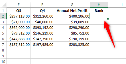
There are two ways you can continue from here. You can either type the IF function directly in the cell, or you can click the Formulas tab, click the Logical option in the Function Library group, and then click the IF option from the drop-down menu.
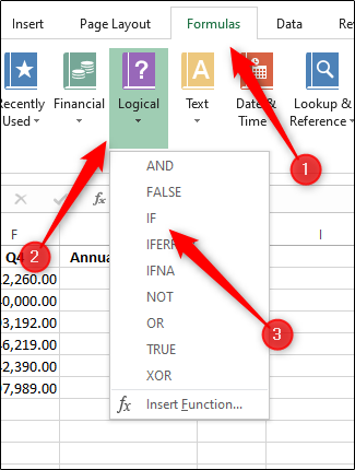
Now, the Function Arguments window will appear. There are three values here we need to input.
- Logical_test: Any value that can be evaluated as true or false.
- Value_if_true: The value that is returned if Logical_test is determined to be true.
- Value_if_false: The value that is returned if Logical_test is determined to be false.
Here are the values we will input in our example.
- Logical_test: G2>200000
- Value_if_true: “A”
- Value_if_false: “B”
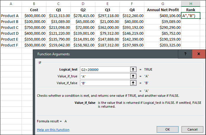
Enter the required information and then click OK. Excel will run the logical test and return the appropriate value.
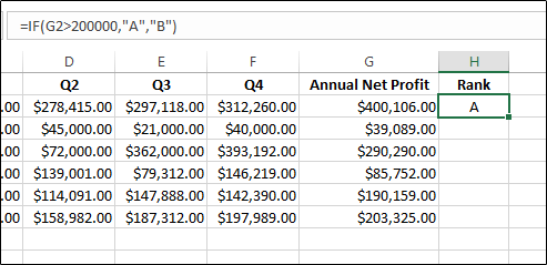
You can now see that, based on our data, it has been determined that our first product is rank A, as it netted a profit of over $200,000. To quickly determine the ranking of the other products, you can click and drag the bottom right corner of the H2 box down to the necessary row (H7 in our example).
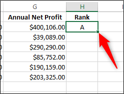
The formula will automatically adjust itself to reflect the data in each row.
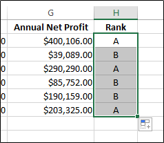
This is especially useful for companies needing to quickly determine results for a long list of items.
4. Determining outcomes with IF
It’s all in the name. IF (x), then do (y). Otherwise, do (z). Performing this logical test to determine an outcome based on a true or false scenario can save a tremendous amount of time, especially when you’re faced with a long list of items to work through.
This is just one of the many Excel formulas used by data analysts on a day-to-day basis. To further your expertise in data analytics, try out our free introductory short course.
You may also be interested in the following video, in which our own senior data scientist, Tom, goes over some of the most important Excel functions for data analysts:
If you found this tutorial helpful, you may want to explore more of our Excel guides. Check out these articles:
