Checkboxes in Excel are a very useful tool to make your spreadsheets more interactive for users. They are an instantly recognizable form control that users will immediately know how to use.
In this article, we’ll show you how to insert a checkbox in Excel. You will also learn how to edit the checkbox properties, and write formulas to work with the checkbox selections.
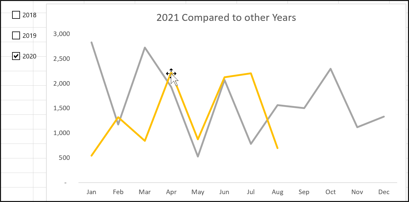
The example used in this tutorial is to use checkboxes to make an interactive chart. This is a very useful scenario for using checkboxes. It takes the chart beyond the static boring charts created by many.
You can learn even more Excel analysis skills with CareerFoundry’s free 5-day data short course.
In this checkbox tutorial, I’ll cover:
- What is a checkbox in Excel?
- How to insert a checkbox in Excel
- How to modify the properties of a checkbox
- Using formulas with checkboxes
You can download the Excel workbook to follow along with the examples in this article.
So, let’s dive in and learn how to use checkboxes in Excel.
1. What is a checkbox in Excel?
A checkbox is a control in Excel that is most commonly used when creating forms and checklists. It is a simple and effective way of creating interaction for the users of your spreadsheets.
Checkboxes enable a user to make multiple selections. If you want a control to only allow a single selection, you want an option button control.
2. How to insert a checkbox in Excel
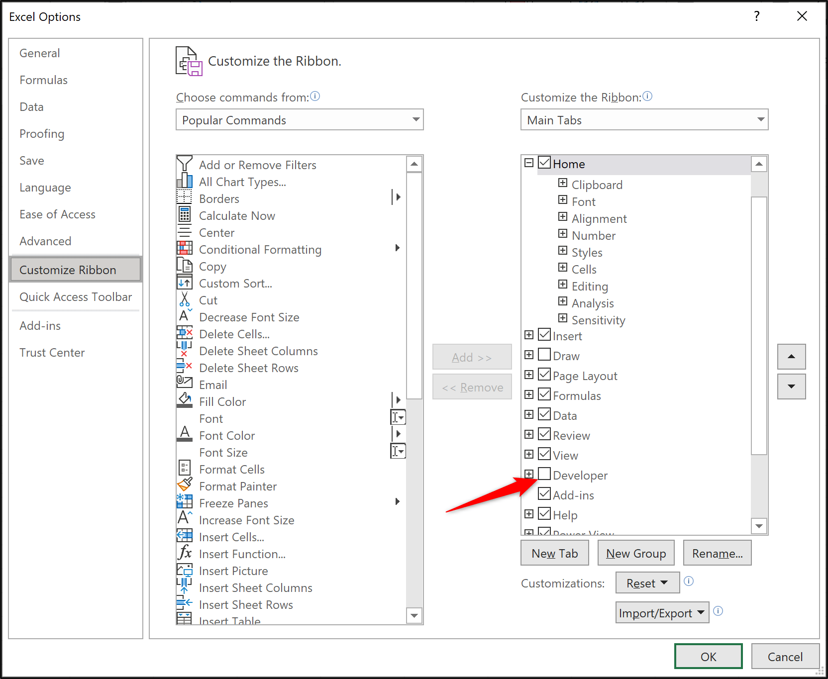
To insert a checkbox, you first need to ensure that the Developer tab is visible on the Ribbon of Excel.
To show the Developer tab:
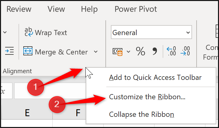
- Right click anywhere on the Ribbon and click Customize the Ribbon.

- Check the box for the Developer tab in the list on the right. Click Ok.
With the Developer tab visible, we can now insert a checkbox. But first, let’s have a quick look at why we want a checkbox.
In the following image, we have sales data for the months of four years. 2021 is incomplete as the year is just finishing.
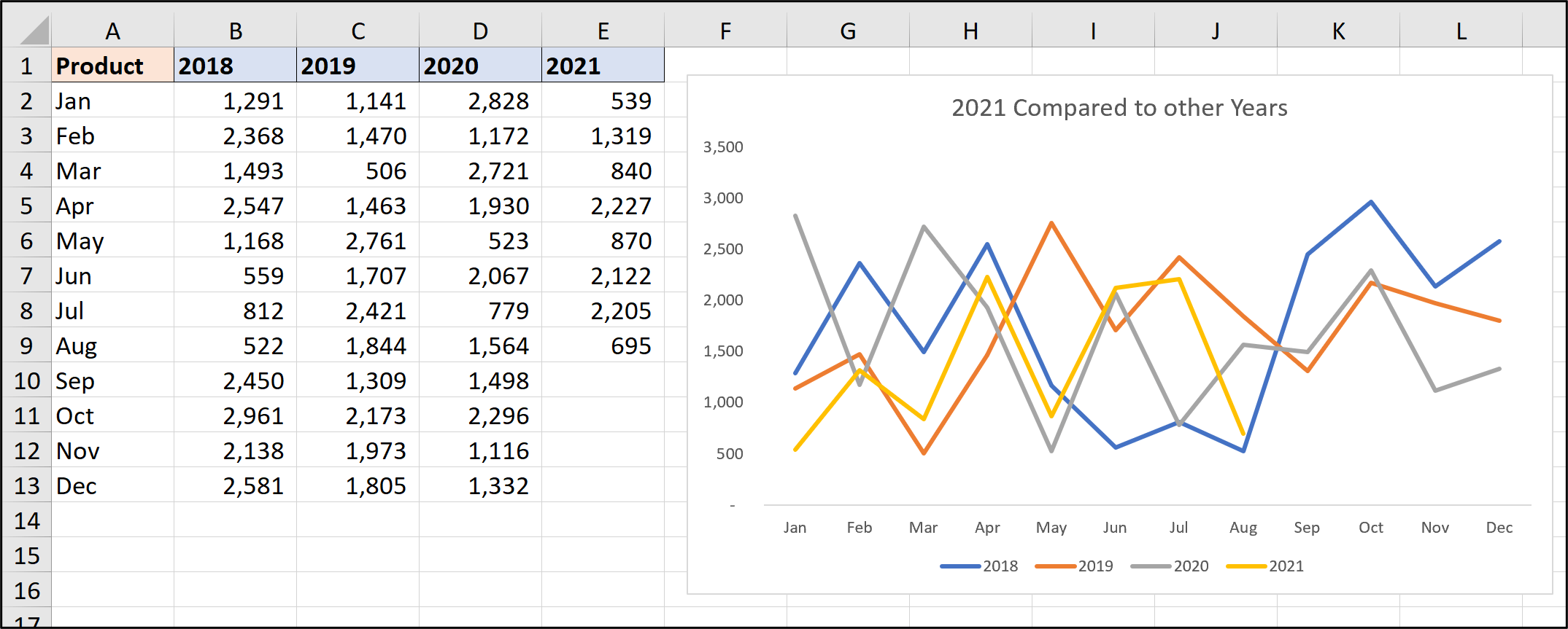
Having all four years in the line chart is a little messy and hard to read. So, let’s insert checkboxes and enable the user to select the year(s) to compare 2021 against.
To insert a checkbox in Excel:
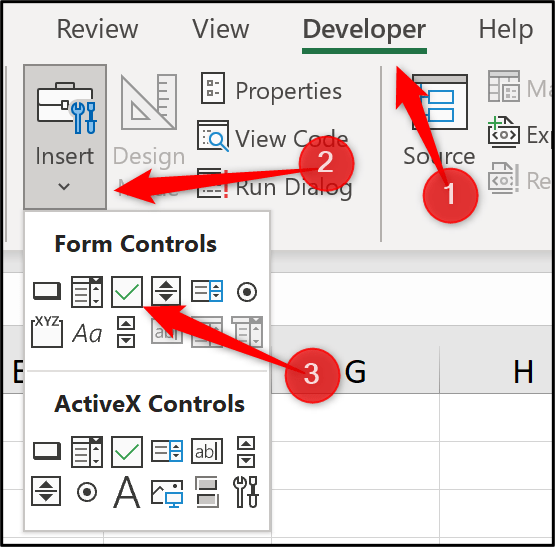
- Click Developer on the Ribbon.
- Click Insert and click the Check Box (Form Control) from the menu.

- Click on the sheet where you want the check box to appear.
- Click on the text of the checkbox to edit it. We will use the names of the years as labels, starting with “2018”.
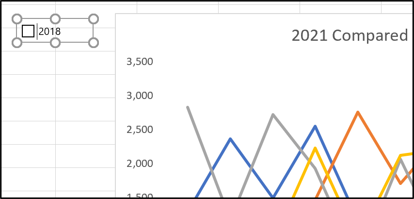
I have moved the chart further down the worksheet from the previous image. This is to make room for some formulas that are coming soon.
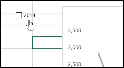
If you click on the sheet off the checkbox, you will no longer be in edit mode and the checkbox is now clickable. If you click it, the box will check. This does not perform any purpose yet (we will need the formulas).
The following image shows the hand cursor indicating the checkbox is ready to be checked and unchecked.
Repeat this task to create two more checkboxes on the sheet, and label them “2019” and “2020”.
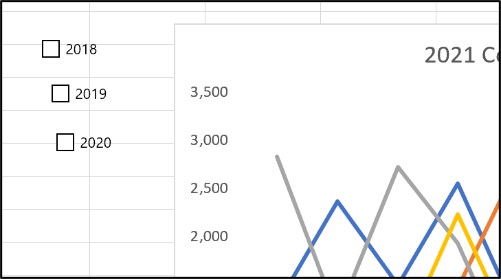
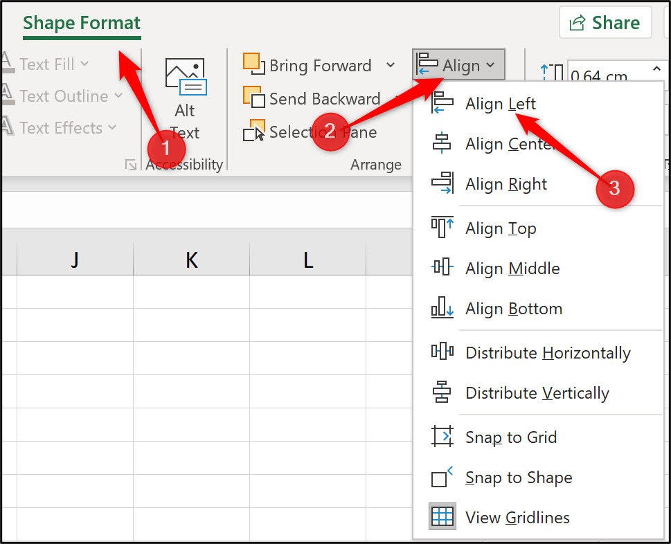
These checkboxes are quite disorganized. To align their left edges perfectly:
- Right-click the first checkboxes to select it.
- Press and hold Ctrl and left-click the other two checkboxes.
- Click the Shape Format tab on the Ribbon, click Align and Align Left.
- Click Align and Distribute Vertically to evenly space the checkboxes.
3. How to modify the properties of a checkbox
To modify the properties of a checkbox:
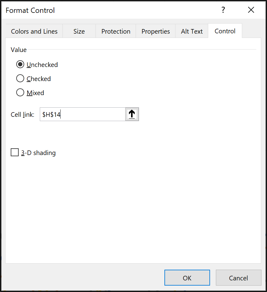
- Right-click on the checkbox and click Format Control.
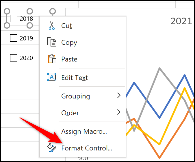
There are a few useful properties in this window. Let’s begin with the most important property: the Cell link.
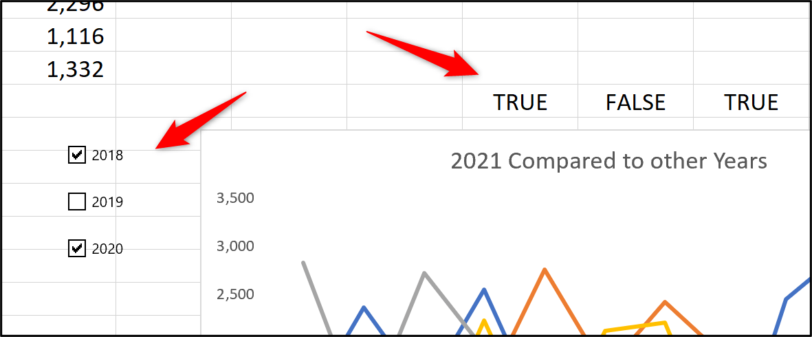
Each checkbox needs to be linked to a cell in the workbook. When a user interacts with a checkbox by either checking or unchecking it, the status of the checkbox will appear in the cell it is linked to.
- Click on the Control tab, and click in the Cell link field.
- Click the cell you want to link it to and click Ok.In this example, the 2018 checkbox has been linked to cell H14. This will be just below the chart range we will create with our formulas.

- Repeat the cell link for the other two checkboxes. Link the 2019 checkbox to cell I14 and 2020 to cell J14.
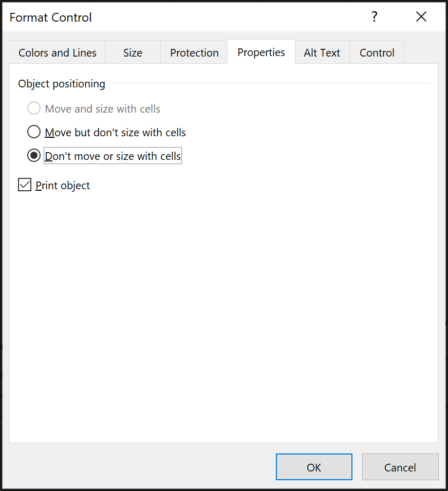
Another property of the checkboxes which is not as important, but can be very useful, is to stop them moving or resizing when rows and columns are added, deleted, and resized.
This setting can be found on the Properties tab of the Format Control window for each checkbox.
4. Using formulas with checkboxes
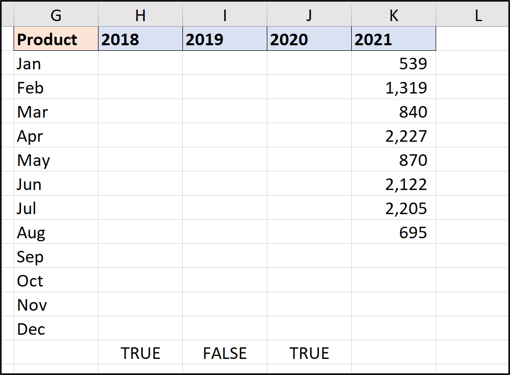
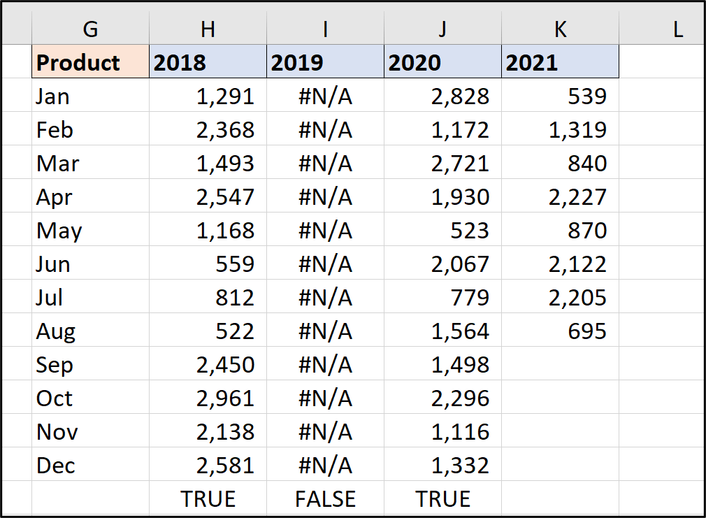
The final step to get the checkboxes to control the chart, is to create a new chart source range and use formulas to display the year’s sales value only if the checkbox is checked.
- Prepare the chart area as shown in the following image. The headers, month labels, and values for 2021 have all been copied over to the new chart range.

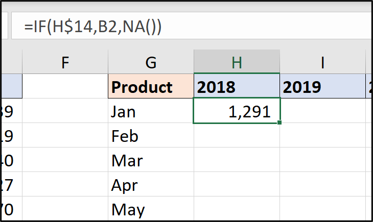
- In cell H2, write the following formula to show the sales value if the 2018 checkbox is checked, otherwise display the NA() error (this prevents the chart plotting the data).

- Fill the formula to range I2 and J2. Then fill the formula down to row 13 to complete the chart range.

- Adjust the chart’s data source to use the new calculated range, or re-create the chart (whatever you find easiest). Now, when you interact with the checkboxes the chart changes.

- Hide the gridlines on the sheet, to improve the look of the checkboxes. To do this: click View and uncheck the Gridlines box.
- Continue to make improvements to the chart and also the layout of the checkboxes to fit your needs.
This was a simple example with a chart that will hopefully give you ideas of where you could implement checkboxes in your Excel reports, forms, and models.
You can use any formula from the result of a checkbox and they provide a great way of creating interaction with the users of your spreadsheets.
For a hands-on introduction to the field of data analytics, try out this free five-day short course. And, for more Excel tutorials, check out the following:

