The COUNTIFS function in Excel is one of the best functions to know.
Whether you’re considering a career as a data analyst or just want to hone your expertise in Excel, I highly recommend that you master this function. It is very versatile and has helped me accomplish a wide variety of tasks over the years.
The COUNTIFS function is used to count only the values in a list that meet specified criteria. For example, only count the orders for a specific product, or only count the exam scores where the result was 70 or higher.
In this tutorial, we’ll show you how to use the COUNTIFS function. We’ll also provide a few examples of using COUNTIFS in different scenarios .
We’ll cover:
- What is the COUNTIFS function and why use it?
- How to use the COUNTIFS function (step-by-step)
- Things to consider when using the COUNTIFS function
- Testing numbers with the COUNTIFS function
- Testing multiple conditions with COUNTIFS
- Using cell references with COUNTIFS
- Combine text and cell references in your criteria
- COUNTIFS function with date conditions
So: let’s dive into the COUNTIFS function.
1. What is the COUNTIFS function and why use it?
The COUNTIFS function was introduced in 2007 to be the successor to the COUNTIF function in Excel.
The COUNTIF function can count values when a single condition is met. However, COUNTIFS can test a single or multiple conditions. So, it is useful to be aware of the COUNTIF function, but COUNTIFS is far superior.
If you’re using Excel for data analysis, then this function is incredibly useful. Along with sum and average, count is another common requirement when analyzing data.
With the COUNTIFS function, you can count the values that meet any criteria that you specify.
The COUNTIFS function requires only two arguments, but can handle many more optional criteria.
=COUNTIFS(criteria_range1, criteria1, [criteria_range2], [criteria2], …)
Criteria range 1: This is the range that is being tested.
Criteria 1: The criteria to apply to the criteria range. This can be a number, text, a cell reference or another function. We will see some of these examples in this tutorial.
[Criteria range 2, Criteria 2], …: Additional ranges and the criteria to apply to them. Using these extra criteria is optional.
2. How to use the COUNTIFS function (step-by-step)
The examples in this tutorial use the table of data as shown in the following example. You can use this Excel workbook to follow along with the examples.
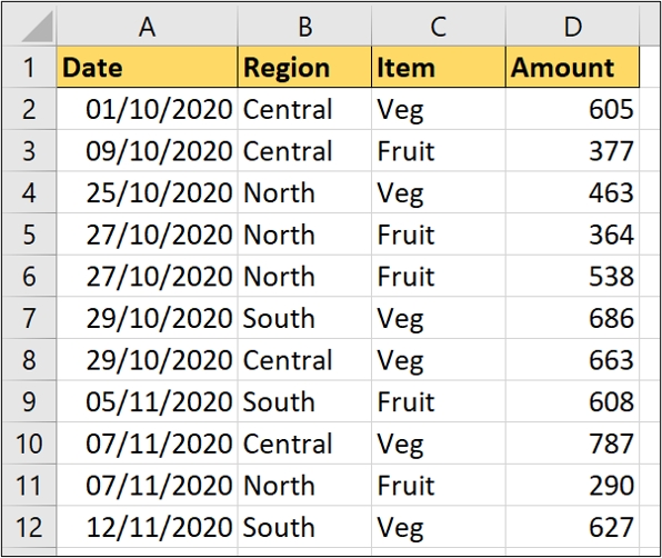
In this first example, we want to use the COUNTIFS function to count the number of orders from the region Central.
Click in the cell where you would like to return the result, and enter the following formula.
=COUNTIFS($B$2:$B$12,”Central”)
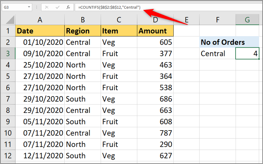
Range B2:B12 has been specified as the criteria range. The criteria “Central” has been typed inside the double quotation marks (“) to denote written text.
The criteria is always written into COUNTIFS inside double quotation marks when text characters are used. When the criteria is a number, cell reference, or a function then the double quotations are not required.
3. Things to consider when using the COUNTIFS function
There are a few things to be aware of when using COUNTIFS.
- When testing multiple criteria, every condition must be met for a value to be counted.
- The number of rows and columns must be the same for each criteria range specified.
- When testing text, COUNTIFS will perform an exact match. However, it is not case-sensitive.
- The ampersand (&) can be used to make criteria from a combination of text and cell references. Examples of this are shown in section seven.
- The asterisk (*) and question mark (?) wildcard characters can be used for partial matches.
- The Tilde (~) character can be used in front of the asterisk or question mark, if you need to count those specific characters.
4. Testing numbers with the COUNTIFS function
The previous example, saw the COUNTIFS function using a text string as its criteria. Let’s now look at an example that tests numeric values.
The following formula returns the number of orders valued at 500 or more.
=COUNTIFS($D$2:$D$12,”>=500”)

In this example, range D2:D12 is specified as the criteria range. The criteria is still entered within double quotation marks, because the “>=” characters are used.
The logical operators “<” for less than and “<>” for not equal to, can also be used when specifying the criteria.
5. Testing multiple conditions with COUNTIFS
Remember, the COUNTIFS function can handle multiple conditions (up to 127 conditions). This makes it superior to the legacy COUNTIF function.
So, let’s combine the two previous examples into one formula. This formula counts the orders that are Central and also greater than or equal to 500.
=COUNTIFS($B$2:$B$12,”Central”,$D$2:$D$12,”>=500”)
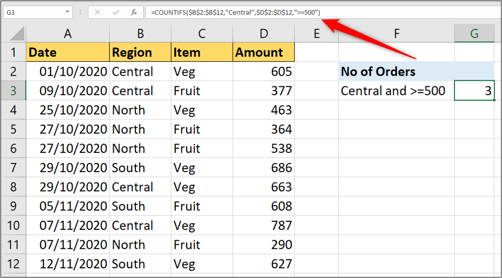
Ensure that the number of rows and columns of each criteria range are the same when using multiple conditions in the COUNTIFS function.
6. Using cell references with COUNTIFS
All of the examples so far have demonstrated the criteria being entered directly into the COUNTIFS function.
Formulas can be made more dynamic by referencing other cells that contain the criteria.
In this formula, the criteria for range B2:B12 has been entered into cell F3 and the criteria for range D2:D12 has been entered into cell F4.
=COUNTIFS($B$2:$B$12,F3,$D$2:$D$12,F4)
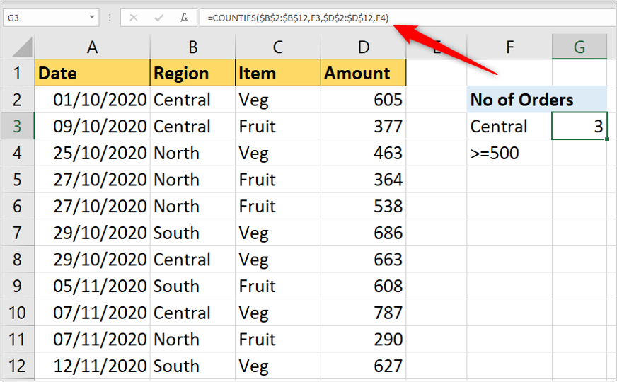
The formula result will change when the values in cells F3 and F4 are changed.
7. Combine text and cell references in your criteria
Taking the previous example further, entering the logical operators such as “>=” into cell F4 with the value is not ideal. Not all Excel users will be comfortable with this.
The ampersand (&) can be used to combine text and a cell reference together to form criteria.
This formula expands on the previous example by using the ampersand to join the text string “>=” and cell F4.
=COUNTIFS($B$2:$B$12,F3,$D$2:$D$12,”>=”&F4)
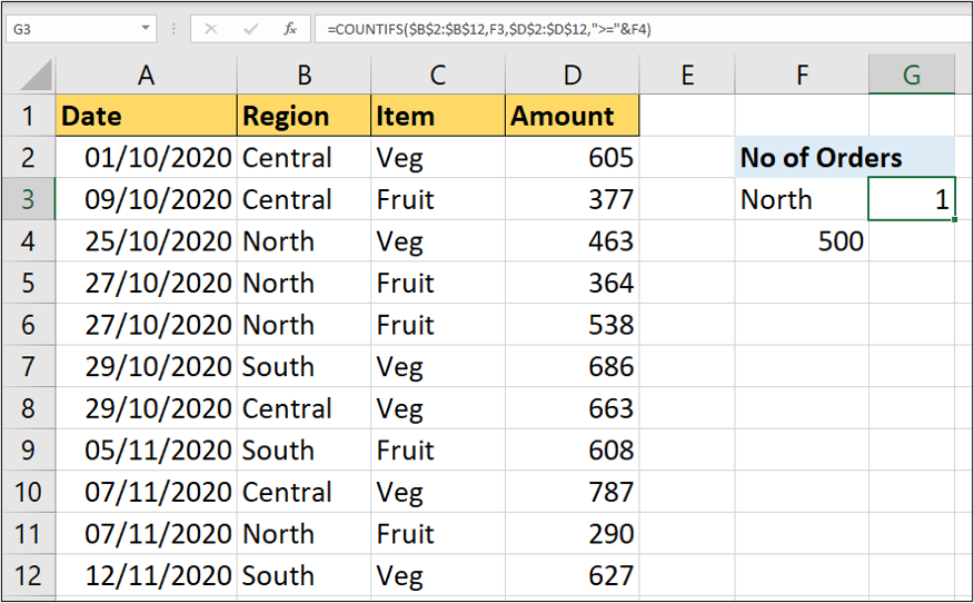
Now, users can simply change the text in cell F3 or the number in cell F4 to update the formula criteria.
8. COUNTIFS function with date conditions
Performing analysis on dates is very commonplace. So, let’s look at examples of the COUNTIFS function with date conditions.
The following formula counts the orders since the date entered into cell F3, and for the region entered into cell F4.
=COUNTIFS($A$2:$A$12,”>=”&F3,$B$2:$B$12,F4)
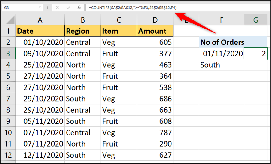
The ampersand was used to join the “>=” operators and the reference to cell F3 like in example 5, as dates are numbers also. However, ensure that the value in cell F3 is recognised as a date.
If you want to enter the date condition directly into the formula instead of using a cell reference, you can enter the date into the criteria like in example 2.
=COUNTIFS($A$2:$A$12,”>=01/11/2020”,$B$2:$B$12,F4)
Final thoughts
Excel formulas are an extremely handy tool for anyone working with data—especially data analysts. For a hands-on introduction to the field of data analytics, try out this free five-day short course. And, for more Excel tutorials, check out the following:
